Economics: where inequality comes from

Two zoo models give two very different answers to “why is wealth unequal?”. In the Boltzmann exchange agents are identical and trade one unit of money at random: inequality comes from chance alone, and settles at a Gini of about one half. In the Bouchaud-Mezard model wealth also earns random returns: the richer earn more in absolute terms, and the distribution grows a power-law tail whose weight depends on how much the agents trade with each other.

Start a project from either with modelly zoo copy kinetic_wealth my_economy (the same command in bash and PowerShell).

Build and run: chance alone

A thousand agents start with five units each. Every step, each agent is paired with another and one of the two, chosen by a coin, gives one unit if it has one.

import numpy as np
import matplotlib.pyplot as plt

from modelly.zoo.kinetic_wealth.model import KineticScenario, KineticWealth

model = KineticWealth(KineticScenario(rng=1, n=1000, money=5, steps=600))
model.run()
gini = model.datacollector.get_model_vars_dataframe()
print(f"Gini after {model.scenario.steps} steps: {gini.iloc[-1, 0]:.3f}")
print(f"Gini of the stationary law:        {model.stationary_gini():.3f}")

Gini after 600 steps: 0.558
Gini of the stationary law:        0.545

Plot: the Boltzmann-Gibbs distribution

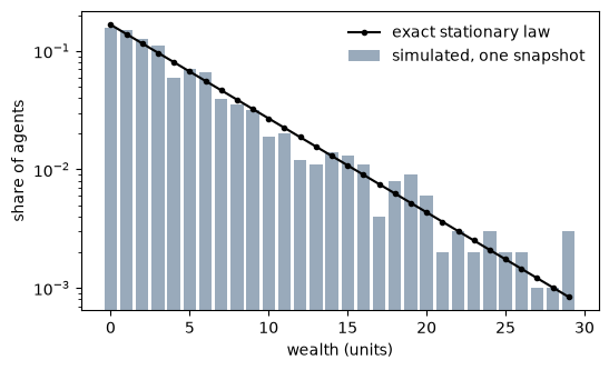
Every configuration of the money with the same total is equally likely in the long run, so the wealth of one agent follows a distribution close to the exponential, P(w) ~ exp(-w / 5).

exact = model.stationary_distribution()
counts = np.bincount(model.wealth, minlength=exact.shape[0]) / model.scenario.n
fig, ax = plt.subplots(figsize=(6, 3.5))
ax.bar(np.arange(30), counts[:30], color="#9ab", label="simulated, one snapshot")
ax.plot(np.arange(30), exact[:30], "k.-", label="exact stationary law")
ax.set_yscale("log")
ax.set_xlabel("wealth (units)")
ax.set_ylabel("share of agents")
ax.legend(frameon=False);

Analysis: returns on wealth create a heavy tail

In the Bouchaud-Mezard model each agent’s wealth is multiplied by a random return of volatility sigma and flows toward the mean at rate J. The stationary distribution of wealth relative to the mean is inverse-gamma with shape 1 + 2 J / sigma^2: the larger sigma^2 / J, the heavier the tail and the higher the Gini.

from modelly.zoo.bouchaud_mezard.model import BouchaudMezard, BouchaudMezardScenario

fig, ax = plt.subplots(figsize=(6, 3.5))
for ratio in (0.5, 1.0, 1.5):
    bm = BouchaudMezard(BouchaudMezardScenario(rng=2, n=2000, volatility=np.sqrt(ratio), steps=1500))
    bm.run()
    w = np.sort(bm.wealth)[::-1]
    share = np.arange(1, w.shape[0] + 1) / w.shape[0]
    ax.loglog(w, share, label=f"sigma^2/J = {ratio}, Gini {bm.datacollector.get_model_vars_dataframe().iloc[-1, 0]:.2f}")
ax.set_xlabel("wealth relative to the mean")
ax.set_ylabel("share of agents at least this rich")
ax.legend(frameon=False);

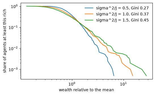
On a log-log plot the tail of the inverse-gamma law is a straight line of slope -2 J / sigma^2: richer agents are much more common than in the Boltzmann world.

Going further

• Give the agents a saving propensity in the Boltzmann exchange and watch the Gini fall.

• Make J a network: exchange only with trading partners.

• The order book is the zoo’s market-microstructure model: its returns have fat tails too, for a different reason.