Energy: how rooftop solar spreads

The Bass model is the standard description of how a new technology spreads: some households adopt because of advertising and subsidies (the innovation coefficient p), most because people they know have adopted (the imitation coefficient q). This tutorial runs the Bass diffusion model from the zoo, compares it with the Bass equation and asks how much the structure of a social network slows adoption down.

Start your own project from it with modelly zoo copy bass_diffusion my_solar (the same command in bash and PowerShell).

Build and run

Five thousand households; a step is a tenth of a year. With mixing="well-mixed" every household sees the adoption share of the whole population, as in Bass’s original model.

import numpy as np
import matplotlib.pyplot as plt

from modelly.zoo.bass_diffusion.model import BassDiffusion, BassScenario, bass_curve

scenario = BassScenario(rng=3, households=5000, innovation=0.03, imitation=0.38)
model = BassDiffusion(scenario)
model.run()
frame = model.datacollector.get_model_vars_dataframe()
frame.iloc[::40]

	time	adoption
0	0.0	0.0000
40	4.0	0.2370
80	8.0	0.6456
120	12.0	0.9054
160	16.0	0.9812
200	20.0	0.9948

Plot: the S-curve against the Bass equation

years = frame["time"].to_numpy()
fig, ax = plt.subplots(figsize=(6, 3.5))
ax.plot(years, frame["adoption"], label="agent-based, well mixed")
ax.plot(years, bass_curve(years, 0.03, 0.38), "k--", label="Bass equation")
ax.set_xlabel("years")
ax.set_ylabel("share of households adopted")
ax.legend(frameon=False);

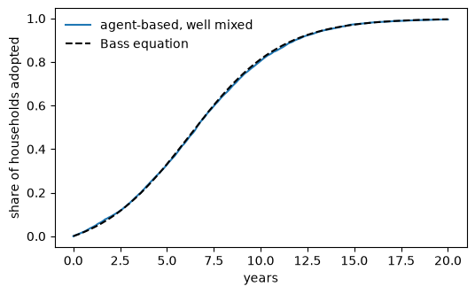
The yearly number of new adopters peaks at t* = ln(q / p) / (p + q):

new = np.diff(frame["adoption"].to_numpy()) / scenario.dt
print(f"peak of the simulated adoption rate: {years[1:][np.argmax(new)]:.1f} years")
print(f"Bass prediction:                     {np.log(0.38 / 0.03) / 0.41:.1f} years")

peak of the simulated adoption rate: 6.6 years
Bass prediction:                     6.2 years

Analysis: does the network matter?

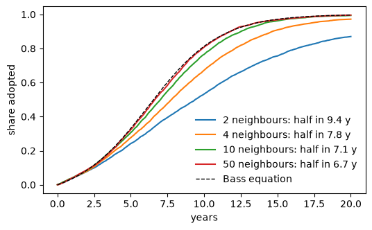
On a random network each household sees only its neighbours. With few neighbours, clusters of non-adopters see fewer adopters than the population average, and imitation is slower.

fig, ax = plt.subplots(figsize=(6, 3.5))
for degree in (2, 4, 10, 50):
    network = BassDiffusion(BassScenario(rng=3, mixing="network", degree=degree))
    network.run()
    curve = network.datacollector.get_model_vars_dataframe()
    half = curve["time"][curve["adoption"] >= 0.5].iloc[0]
    ax.plot(curve["time"], curve["adoption"], label=f"{degree} neighbours: half in {half:.1f} y")
ax.plot(years, bass_curve(years, 0.03, 0.38), "k--", lw=1, label="Bass equation")
ax.set_xlabel("years")
ax.set_ylabel("share adopted")
ax.legend(frameon=False);

Going further

• Read a real social network with modelly.space.networks.read_edge_list.

• Make innovation depend on a subsidy that starts in a given year.

• Calibrate p and q on an adoption series by least squares on bass_curve.