Epidemiology: who gets infected, and how many

How many people will an epidemic infect, and in which age groups? This tutorial runs the age-structured SEIR model from the zoo, checks it against the final-size relation, and uses the contact matrix to compare two interventions.

Start a project from it with modelly zoo copy age_seir my_epidemic (the same command in bash and PowerShell).

Build and run

A hundred thousand people in three age groups. contacts[a][b] is the mean number of contacts a member of group a has with members of group b per day; it is reciprocal, so N[a] * C[a, b] == N[b] * C[b, a]. In a real study it comes from a contact survey, or from a synthetic population through modelly.space.networks.contact_matrix.

import numpy as np
import matplotlib.pyplot as plt

from modelly.zoo.age_seir.model import AgeSEIR, SEIRScenario, State

GROUPS = ("children", "adults", "seniors")
scenario = SEIRScenario(rng=42)
model = AgeSEIR(scenario)
print(f"R0 = {model.r0():.2f}")
model.run()
model.datacollector.get_model_vars_dataframe().iloc[::50]

R0 = 2.17

	S	E	I	R
0	99970	0	30	0
50	92602	2032	1747	3619
100	27623	2457	4600	65320
150	22360	34	69	77537
200	22323	1	0	77676
250	22323	0	0	77677
300	22323	0	0	77677
350	22323	0	0	77677
400	22323	0	0	77677

The population is a table of cohorts, one row per (age group, state), so the run costs the same for a hundred thousand people as for a hundred:

model.people.to_dataframe()

	count	group	state
0	2187	0	0
1	17813	0	3
2	10883	1	0
3	49117	1	3
4	9253	2	0
5	10747	2	3

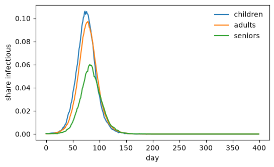
Plot: the epidemic curve

model = AgeSEIR(scenario)
infectious = []
for _ in range(scenario.steps):
    model.step()
    infectious.append(model.counts()[:, State.I] / model.sizes)
fig, ax = plt.subplots(figsize=(6, 3.5))
ax.plot(np.array(infectious), label=GROUPS)
ax.set_xlabel("day")
ax.set_ylabel("share infectious")
ax.legend(frameon=False);

Check: the final-size relation

Over the whole epidemic the share s_a of group a that escapes infection solves log(s_a) = log(s0_a) - (beta / recovery) * sum_b C[a, b] * (1 - s_b). final_size() solves it; the simulated attack rates agree to within the sampling noise.

import pandas as pd

pd.DataFrame(
    {"simulated": model.attack_rate(), "final-size relation": model.final_size()},
    index=GROUPS,
).round(3)

	simulated	final-size relation
children	0.889	0.889
adults	0.815	0.815
seniors	0.541	0.538

Analysis: which intervention?

Halving the contacts among children (closing schools) and halving every contact of the seniors (shielding) reduce R0 differently, and protect different groups.

contacts = np.array(scenario.contacts)
schools = contacts.copy()
schools[0, 0] /= 2
shielding = contacts.copy()
shielding[2, :] /= 2
shielding[:, 2] /= 2
rows = {}
for label, matrix in {"none": contacts, "schools": schools, "shielding": shielding}.items():
    run = AgeSEIR(SEIRScenario(rng=42, contacts=tuple(map(tuple, matrix))))
    run.run()
    rows[label] = [run.r0(), *run.attack_rate()]
pd.DataFrame(rows, index=["R0", *GROUPS]).T.round(3)

	R0	children	adults	seniors
none	2.165	0.891	0.819	0.537
schools	1.961	0.773	0.803	0.528
shielding	2.115	0.873	0.793	0.263

Going further

• Build the contact matrix from a synthetic population with households, schools and workplaces; see Networks and the layered epidemic example.

• Make beta a function of time to model a lockdown.

• Fit beta to an observed epidemic curve.